In this section, we delve into the mathematical methods used during backtesting to determine statistical significance and validity. Historical backtests perform single test strategies known as t-tests and compare trading strategies using Sharpe ratios.
Single Tests and Sharpe Ratios
In order to test if a trading strategy is profitable, statistical analysts perform statistical hypothesis tests called t-tests. The null hypothesis, the strategy simulated under, maintains that the expected returns are equal to zero. The alternative hypothesis attempts to disprove the null in favor of the belief that expected returns are different from zero. The alternative hypothesis, therefore, is two-sided. If statisticians can prove that expected returns are different from zero, they may reject the null hypothesis and accept the alternative hypothesis. In doing so, they have effectively found a profitable trading strategy that is different from zero in either the positive or negative direction.
Given a sample of data consisting of historical returns, the mean (µ) and standard deviation (σ) of the sample can be measured. The t-test assumes that the test statistic follows a normal distribution, so the distribution would contain T − 1 degrees of freedom. By constructing the t-test ratio, which is shown in Figure 15, statisticians may test the null hypothesis that the average return is zero; the result of the hypothesis test will deduce whether the investment strategy is statistically significant.

The Sharpe ratio is a metric of risk-adjusted return, taking into account both return and volatility, and is directly linked to the t-test ratio. A given trading strategy with high return and high volatility may be seen as less effective than a strategy with lower return and low volatility under the Sharpe ratio. The period and frequency of the tests between the two strategies must be standardized. Sharpe ratios allow traders to perform risk/reward analysis for their trading strategies and is an important aspect of backtesting. The Sharpe ratio is defined as the mean (µ) divided by the standard deviation (σ), as shown in Figure 16. Intuitively, the mean represents return and the standard deviation represents volatility. By setting the t-ratio and Sharpe Ratio equal, the Sharpe ratio can be set equal to the t-ratio/ √T. Due to the fact that the T is fixed under a normal distribution, there is a direct positive correlation between the t-ratio and Sharpe ratio; as the Sharpe ratio increases, the t-ratio increases, as well. A higher Sharpe ratio implies that there is a higher significance level for a trading strategy.

The Sharpe ratio can be used in tandem with the t-ratio to compare trading portfolios. Portfolios with higher Sharpe ratios generate higher excess return per unit of volatility. An efficient frontier occurs when a portfolio generates higher returns for a defined level of risk, which is illustrated in Figure 17. An Inefficient frontier occurs when a portfolio is associated with higher risk and lower returns.

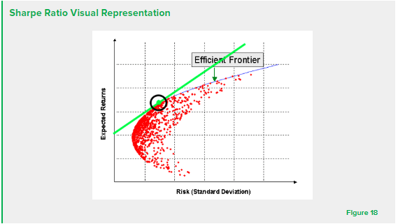
Each data point in Figure 17 represents a possible trading scenario. Given this model, statisticians can locate the ideal trade with the highest possible Sharpe ratio. This process involves generating a line of tangency called the capital market line, as demonstrated in Figure 18. The tangent portfolio circled in the figure below has the highest possible Sharpe ratio. This point has the highest reward per unit of volatility and is a worthwhile investment for traders.

Efficient backtesting systems are programmed to conduct hypothesis tests and develop Sharpe Ratios for individual trades. The backtester develops optimization models using the capital market line to identify the mathematically ideal trading scenario. While the Sharpe ratio is useful in generating risk/reward ratios, it does not guarantee performance for individual traders. Backtesters must take into account economic events and price movements, too, as was discussed in Chapter 2.
Continue to the next part of our backtester series here.


